
In our Hindsight series, researchers highlight a historical piece of research that was -and is- significant to them. In this post, Kai Chan and Edward Gregr look how at the problem of pattern and scale in ecology informs the choice of training and testing data for models to reach beyond description to prediction. Kai Chan is also a Lead Editor for the journal People and Nature.
As an undergraduate student, I (Kai Chan) marvelled at Simon Levin’s (1992) comprehensive distillation of insights about the multi-causality of pattern and the multiplicity of scale in The problem of pattern and scale in ecology: the Robert H. MacArthur award lecture. I thought, “That man is perfect as president of the Ecological Society of America”. And, “I want that man to be my PhD supervisor.”
Fast-forward two decades, and I can honestly say that no single paper is more important to how I understand the world. Not only because it was the paper that connected me to my PhD supervisor (the best anyone could ever hope for), but because the central point is so crucial, and yet still so underappreciated, to all manner of environmental problems.
Pattern, scale, and multi-causality
Levin’s central point is that all observations of ecosystems are patterns produced by numerous processes operating simultaneously over a wide range of scales. Thus, the observed characteristics of an animal population (e.g., its distribution or a decline in survivorship) are functions of the interplay between climate, vegetation, mutations and genetic sweeps, and the behaviour of the species in question as well as that of other interacting species including pathogens and parasites. And all these factors act at multiple scales and interact differently in different contexts. Sounds straightforward, doesn’t it?
Except that the implications of this complexity are routinely ignored in science, policy, and management. For example, resource development policy generally assumes we need not, and should not, restrict a specific project (like a pipeline or mine) unless we have clear evidence that it is likely to cause an undesirable impact on something protected by law (a ‘valued ecosystem component’, such as an endangered population of salmon). But if there are always multiple processes interacting in a context-dependent way, we may never be able to prove that any single impact or project is the cause, or at least not until it’s too late. Such multi-causality is one of the fundamental concepts anyone working with ecosystems must understand.
Understanding the models you build
The challenges of trying to understand an interacting, multi-causal, dynamic system are what drew me (Edward Gregr) to explore how modelling ecosystems, habitats, and species distributions can support decision-making in resource management. In particular, models of species’ distributions are increasingly common, driven by a management need to assess the impacts of human activities on ecosystems and the species they include. However, building models is one thing, understanding their limitations is quite another.
From a management perspective, a key question is how well do habitat models predict patterns of species’ distributions at different times, or in different places–that is, how transferable is the model, or how good is its forecasting? It is generally accepted that the best way to answer this question of transferability is by comparing the model predictions to an independent set of species observations. However, since independent observations are often not available, models are typically evaluated by using a subset of the data available to build them. Termed cross-validation, this approach generally divides the available observations into several data folds (i.e., subsets) which are then used as ‘training’ and ‘testing’ samples. However, this approach is understood to over-estimate model forecast skill, because the training and testing data are not independent (e.g., Goodall 1972; Yates et al. 2018). The concept of independence is straightforward when considering individual observations within a sample: two observations are statistically independent if one does not affect the probability of the other. But what constitutes independence between sets of observations? And when can cross-validation partition the data so that the data folds are sufficiently independent to legitimately test model forecast skill?
From Levin (1992) to Gregr et al. (2018)
It turns out the ideas of multicausality and patterns across scales are key to these questions (where scale includes both study extent and resolution). We had the opportunity to examine this relationship in detail thanks to a peer-review of our work on predicting kelp distributions (reported in our recent paper in Ecography).
In our study we used purpose-collected field data to train a set of increasingly complex models, and 4 independently collected datasets to test model forecast skill. The testing datasets included one collection of long-term observations and 3 ‘snapshots’ from different years classified from satellite images. In our manuscript, we made two important claims: first, that performance measures based on random cross-validation over-estimate a model’s ability to predict in other contexts (forecasting) compared to independent data validation, and that this performance metric is tied to model complexity. The implication being that overly complex models can have poor forecasting ability because they are overfit to the training data (thus illustrating the classic trade-off between model generality and precision, e.g., Levins 1966).
On peer review we were challenged that the apparent inadequacy of cross-validation may have been due to our use of random cross-validation (which is still widely used, although experts consider it inadequate). The peer reviewer further claimed that block-cross validation—where the collection of observations is divided into independent data folds using known geographic or other distinguishing factors—would prove as effective as independent data evaluation for evaluating transferability. We were not happy to have to redo the analysis, but we embarked on the journey, curious to see if the reviewer was right.
What did we find? Well, first, the re-analysis allowed us to refine some of our methods, leading to more parsimonious models—a nice bonus. But when we did compare the performance metrics from block-cross validation, our results were entirely upheld: blocking made little difference to the cross-validation-based estimates of forecast skill.
While we were vindicated by these findings, we were a bit at a loss as to how best to discuss them. We had a sense from our analysis that the idea of “representativity” (i.e., how well a dataset represents the potential predictive space) was critical to the effectiveness of model forecasts. But how were we to reconcile this with the reviewer’s (and the literature’s) focus on “independence”? Was there still a problem with our analysis? Were the folds from our block-cross-validation still not independent? And how did our study, with a spatially localized dataset, compare with the “big-data” analyses (that combine observations from a wide range of different places and times) where block-cross validation has been used most commonly and with some success (Roberts et al. 2017)?
In the end, we came up with the following ideas about independence, representativity, and their relationship to robust model evaluation. It may not be 100% accurate, but we did not find these ideas discussed collectively anywhere we looked.
Independence, context and complexity
The question of sample independence was the hardest for us to get our heads around. But we eventually realized that what counts as independent at one scale is not independent at another. This is nicely illustrated by considering the difference between Ecology as an experimental exercise, and Landscape Ecology as a study of ecological context (sensu Wagner and Fortin 2005). Typically considered at different scales, these two disciplines represent the two extremes of sample independence: at the experimental scale, we have replicates, samples that are assumed identical so any observed difference can be attributed to a treatment—classic experimental stuff. At the landscape scale, context is critical, and questions focus on differences between systems. Thus, experimental replicates (e.g., a collection of small vegetation plots in a field) are considered independent because the extents of the study do not extend beyond the field of interest (and experimental ecologists are quick to note that any results apply only to similar fields). However, at coarser resolutions (or broader extents), the replicates would be fully dependent because as the study area is broadened, their shared context makes them increasingly similar. If the two samples were moved further apart in this expanded study area, they would become increasingly independent as their ecological contexts diverge. Given the multi-causal (and multidimensional) aspects of ecosystems, myriad factors have the potential to increase the independence between samples: seasonality, year-to-year variability, differences in biodiversity, or human impacts, etc. When studying whole systems, sample independence is thus a function of scale, making sample independence a matter of degree rather than a binary distinction.
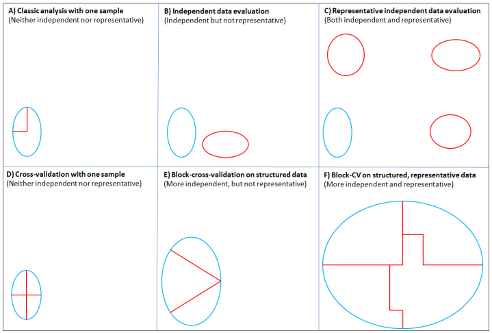
Interestingly, this idea of ecological context also helped us understand the question of representativity, because while shared ecological context makes two samples less independent, it also makes them less representative of the predictive space of interest. We highlight these differences (Fig. 1) using a generalized representation of context on two dimensions (say time and space). The figure shows the methods typically applied to different collections of observational data to partition the training and testing data sets, and how their independence increases as the context for two patterns diverge. However, unless the samples span a significant portion of overall context of interest (e.g., Fig. 1C, F), they are not going to be representative.
In our analysis, our independent testing data were collected at different times and in different ways from the training data, so they were effectively independent in time, providing good representativity across at least one dimension of the predictive space (Fig. 1).
Crucially, our simple models performed better than the more complex ones because they described processes that were persistent across contexts, rather than fitting a pattern unique to the training context (the converse was true for the complex models). We are thus reasonably confident that our simple models are transferable across time. However, we are less confident in the transferability across space, because our testing data came from the same region.
In writing this blog post, we realized that block cross-validation is at its best when applied to a large data set that spans many contexts, giving it a wide diversity of patterns to examine (e.g., Fig. 1F). Although, this assumes an understanding of the data that would allow blocking the data into more-independent samples. When applied to a data set (like ours) from a restricted, independent context (Fig. 1D), blocking the data appears to be ineffective.
Back to the beginning
We started out with the ideas of pattern, scale, and multi-causality, and that’s also where this story ends. Levin pointed out that patterns—as products of multiple processes operating (and interacting) at multiple scales—can and should be analyzed at multiple scales. A model built and tested in one place is likely to be tailored (i.e., fit) to that place in ways that compromise its predictions elsewhere. This could be because the processes driving the pattern are context-dependent. If we want a model to apply more generally across broader spatial (or temporal) extents, we need to ensure that we capture the processes that generate the patterns observed in other contexts, and test it with data that represent those contexts.
It all sounds rather obvious now, perhaps because none of these ideas are new in their own right. But we hope our attempts to bring together these ideas around independence and representativity, cross-validation and independent data evaluation, and model complexity and performance, are helpful for understanding how to evaluate ecological models and their forecasts.
References
Goodall, D. 1972. Building and testing ecosystem models. Mathematical Models in Ecology, ed. JNR Jeffers, 173-94. Oxford: Blackwell.
Gregr EJ, Palacios DM, Thompson A, Chan KMA (2018). Why less complexity produces better forecasts: An independent data evaluation of kelp habitat models. Ecography 0(ja).
Levin SA. 1992. The problem of pattern and scale in ecology: the Robert H. MacArthur award lecture. Ecology. 73(6):1943-67.
Levins R. 1966. The strategy of model building in population biology. American scientist. 54(4):421-31.
Roberts DR, Bahn V, Ciuti S, Boyce MS, Elith J, Guillera-Arroita G, Hauenstein S, Lahoz-Monfort JJ, Schröder B, Thuiller W, Warton DI. 2017. Crossvalidation strategies for data with temporal, spatial, hierarchical, or phylogenetic structure. Ecography. 40(8):913-29.
Wagner, HH, Fortin MJ. 2005. Spatial analysis of landscapes: concepts and statistics. Ecology 86(8):1975-1987.
Yates KL, Bouchet PJ, Caley MJ, et al. 2018. Outstanding challenges in the transferability of ecological models. Trends in Ecology & Evolution.#
 but gives no insight on the model’s forecast skill.")


, block cross-validation could produce independent data folds that improve the confidence in measures of forecast skill.")

Figure 1: Illustration of how different training and testing strategies influence the independence and representativity of the training (blue) and testing (red) datasets. Each box represents the extents of the multidimensional predictive space (e.g., space and time). Ellipses represent sets of observations (i.e., patterns) collected for particular ecological contexts (e.g., a particular place and time).
Panel A: A typical approach to modelling with a single sample. The data are partitioned into a training and a testing data set. This allows tests of model fit (internal validation) but gives no insight on the model’s forecast skill.
Panel B: When an independent sample is available it provides an estimate of forecast skill, but if not sufficiently representative of the predictive space, it will limit the contexts to which the forecast applies.
Panel C: The ideal situation for independent data evaluation, where multiple sets of independent observations span the entire predictive space are available.
Panel D: Cross-validation applied to an independent sample. Our analysis suggests that in this case block cross-validation is no better than random cross-validation.
Panel E: When applied to a larger sample of observations with a detectable structure (red divisions), block cross-validation could produce independent data folds that improve the confidence in measures of forecast skill.
Panel F: The ideal situation for block cross-validation where a large sample spans the predictive space, and structure in the observations can be used to tease out more-independent data folds. In practice, the independence achieved through blocking is often difficult to assess.
